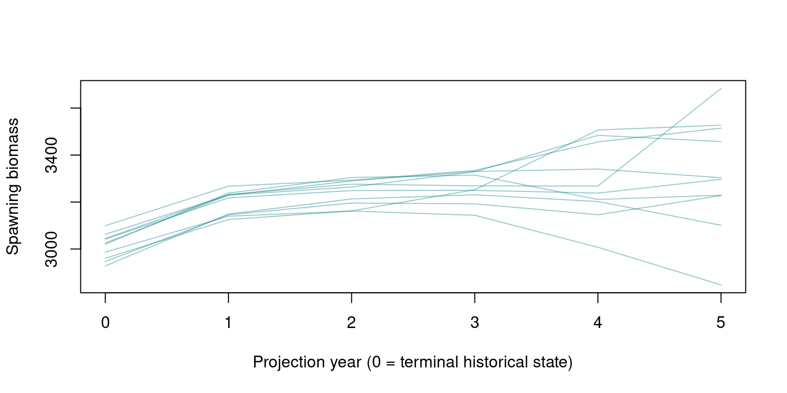
This example carries one opal_obj from a saved fixed-effects assessment through a five-year projection and a save/read round trip. Ten trajectories keep the example quick; they demonstrate the interface and do not provide assessment-quality uncertainty estimates. See the Quickstart for fitting and the saved-fit review for diagnostics.
Load and check the assessment
<opal_obj> fitted
Active parameters: 127
Objective: 1832.412
Fit check: failed  | MCMC check: not run
The saved fit may pass the optimiser’s stopping rule while missing Opal’s stricter gradient check. Continue optimisation from the saved point when needed, with the same model and diagnostic threshold. Tighten the optimiser’s relative objective tolerance so that it does not stop before the gradient check passes. Check after each pass, allowing at most three; this example stops if the checks still fail. Reading alone never refits a model.
for (attempt in seq_len(3L)) {
  if (isTRUE(assessment$validation$fit$passes)) break
  assessment <- opal_fit(
    assessment, n_passes = 1L,
    control = list(eval.max = 10000L, iter.max = 10000L, rel.tol = 1e-10)
  )
}
stopifnot(isTRUE(assessment$validation$fit$passes))
summary(assessment)
<opal_obj> fitted
Active parameters: 127
Objective: 1832.412
Fit check: passed  | MCMC check: not run
This illustrative scenario repeats the final observed annual catch, uses the last ten model years to generate future selectivity, and simulates recruitment deviations from an autoregressive model of the fitted history. These are explicit scenario assumptions that require review for each stock.
set.seed(42)
n_proj <- 5L
n_iter <- 10L
data <- assessment$data

recruitment <- project_rec_devs(
  assessment, uncertainty = "fit", arima = FALSE,
  first_yr = data$last_yr - 9L, n_proj = n_proj, n_iter = n_iter
)
selectivity <- project_selectivity(
  assessment, first_yr = data$last_yr - 9L,
  n_proj = n_proj, n_iter = n_iter
)
future_catch <- array(0, c(n_proj, data$n_season, data$n_fishery))
for (year in seq_len(n_proj)) {
  future_catch[year, , ] <- data$catch_obs_ysf[data$n_year, , ]
}
Recruitment has dimensions [iteration, future year]; selectivity has [iteration, fishery, future year, age]; catch has [future year, season, fishery]. Historical windows use the model-year coordinates in data$first_yr and data$last_yr; the bundled Quickstart uses indices 1–75, rather than calendar years. project_selectivity() uses the stored point report and simulates variation independently by age and fishery; it does not propagate posterior uncertainty in selectivity parameters.
Project and retain the result
uncertainty = "mvn" draws parameters using the Hessian at the fitted point. This path supports fixed-effects models. opal_project() retains the output, future inputs, seed, and source identity inside the assessment. Its seed controls the dynamics draws; the seed above controls recruitment and selectivity generation.
assessment <- opal_project(
  assessment, name = "constant_catch", uncertainty = "mvn", seed = 43,
  n_proj = n_proj, n_iter = n_iter,
  rdev_y = recruitment$rdev_y, sel_fya = selectivity,
  catch_ysf = future_catch, return_hist = TRUE
)
projection <- assessment$derived$constant_catch$result
names(projection)
assessment$derived$constant_catch$uncertainty
The first projected state is the terminal historical state for the same parameter draw. Include this bridge point when plotting a continuous trajectory from the historical period into the future.
spawning_biomass <- vapply(
  projection$dyn, function(draw) as.numeric(draw$spawning_biomass_y),
  numeric(n_proj + 1L)
)
matplot(0:n_proj, spawning_biomass,
        type = "l", lty = 1, col = grDevices::adjustcolor("#00797F", 0.4),
        xlab = "Projection year (0 = terminal historical state)",
        ylab = "Spawning biomass")
Save the assessment and its projection
Changing model configuration through opal_update(), or replacing the source fit or posterior, clears stored projections. Change a label through metadata to preserve compatible results.
Use posterior draws
For an assessment with MCMC, select the uncertainty source explicitly. Recruitment and dynamics consume the same first n_iter retained draws in the same order. Random-effect models require complete joint posterior draws; marginal-only draws and random-effect MVN projections are unsupported.
The following recipe is not executed during documentation builds. Run it after choosing sampling effort and reviewing the MCMC diagnostics.
assessment <- opal_mcmc(assessment, seed = 44, chains = 4, cores = 4,
                        num_warmup = 1000, num_samples = 500)
summary(assessment)
assessment$validation$mcmc

set.seed(45)
recruitment <- project_rec_devs(
  assessment, uncertainty = "mcmc", arima = FALSE,
  first_yr = data$last_yr - 9L, n_proj = n_proj, n_iter = n_iter
)
assessment <- opal_project(
  assessment, name = "posterior_constant_catch", uncertainty = "mcmc",
  seed = 46, n_proj = n_proj, n_iter = n_iter,
  rdev_y = recruitment$rdev_y, sel_fya = selectivity,
  catch_ysf = future_catch, return_hist = TRUE
)
opal_save(assessment, "assessment-projected.rds")