Review an Opakapaka Fit

Review a saved assessment

This vignette upgrades the bundled legacy opal_fit to opal_obj. It examines the portable fixed-effects opakapaka fit created for the Quickstart. It rebuilds the transient RTMB objective to verify the stored objective and obtain predictions, without optimisation.

The bundled fit may have been saved under a different R version. Portable integrity permits that difference while still checking model compatibility and requiring the rebuilt objective to match the saved value.

library(opal)

fit_path <- system.file("extdata", "opaka_quickstart_fit.rds", package = "opal")
if (!nzchar(fit_path)) {
  stop("The bundled opakapaka quickstart fit is unavailable.", call. = FALSE)
}
fit <- opal_read(fit_path)
fit
#> <opal_obj> fitted
#> Active parameters: 127 
#> Objective: 1832.412 
#> Fit check: not run  | MCMC check: not run
summary(fit)
#> <opal_obj> fitted
#> Active parameters: 127 
#> Objective: 1832.412 
#> Fit check: not run  | MCMC check: not run

CPUE fit

plot_cpue(fit)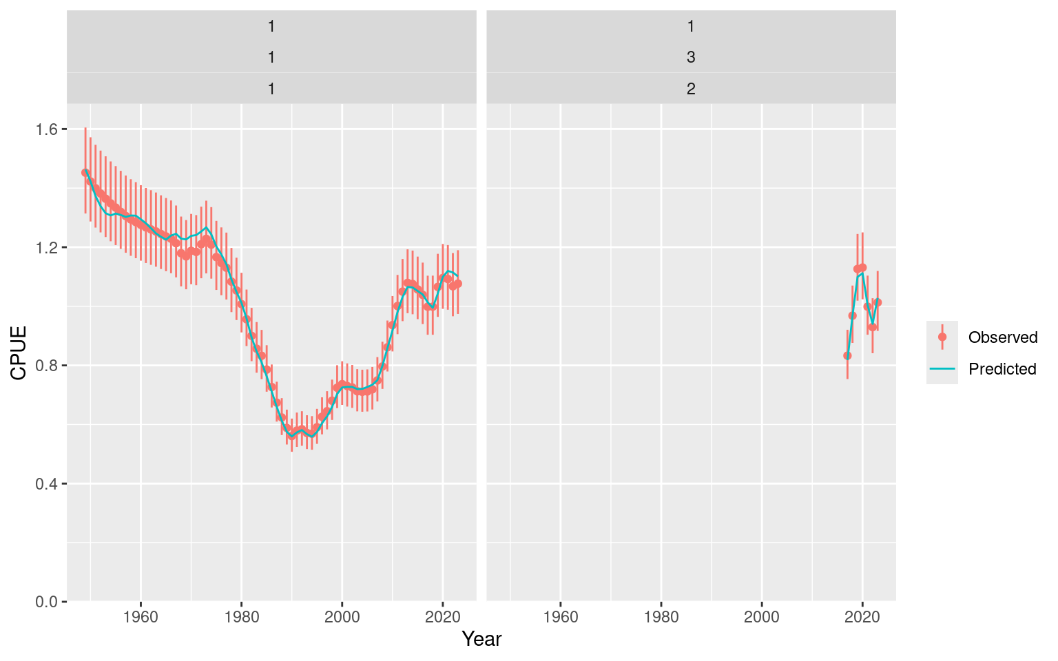

Diagnostics

The compact estimability result and maximum absolute gradient were saved with the fit. They can be inspected without creating a new objective.

list(
  estimability = fit$fit$estimability,
  maximum_gradient = fit$fit$diagnostics$max_gradient
)
#> $estimability
#> $estimability$status
#> [1] "estimable"
#> 
#> $estimability$message
#> [1] "All 127 active fixed-effect parameters are estimable."
#> 
#> $estimability$n_parameters
#> [1] 127
#> 
#> $estimability$n_non_estimable_combinations
#> [1] 0
#> 
#> $estimability$implicated_parameters
#> character(0)
#> 
#> 
#> $maximum_gradient
#> [1] 0.003773483

Refresh the reusable fit checks with opal_check(). The stage remains fitted whether checks pass or fail; inspect the validation record before interpreting the assessment.

fit <- opal_check(fit, scope = "fit")
fit$validation$fit$metrics
#> $convergence
#> [1] 0
#> 
#> $max_gradient
#> [1] 0.003773483
#> 
#> $positive_hessian
#> [1] TRUE
#> 
#> $inside_bounds
#> [1] TRUE
#> 
#> $valid_population
#> [1] TRUE
#> 
#> $biology
#> $biology$passes
#> [1] TRUE
#> 
#> $biology$checks
#>  initial_equilibrium      harvest_penalty           population 
#>                 TRUE                 TRUE                 TRUE 
#>            mortality             maturity   spawning_potential 
#>                 TRUE                 TRUE                 TRUE 
#>               weight          selectivity            steepness 
#>                 TRUE                 TRUE                 TRUE 
#>          recruitment      spawning_output              harvest 
#>                 TRUE                 TRUE                 TRUE 
#>            depletion catch_reconstruction 
#>                 TRUE                 TRUE 
#> 
#> $biology$metrics
#> $biology$metrics$initial_penalty
#> [1] 0
#> 
#> $biology$metrics$total_penalty
#> [1] 0
#> 
#> $biology$metrics$max_harvest
#> [1] 0.09746102
#> 
#> $biology$metrics$max_relative_catch_error
#> [1] 6.704798e-10
summary(fit)
#> <opal_obj> fitted
#> Active parameters: 127 
#> Objective: 1832.412 
#> Fit check: failed  | MCMC check: not run

The bundled legacy fit’s maximum gradient can exceed the default 0.001 tolerance even with optimiser convergence code zero. That is a failed diagnostic check, not a read or migration failure. This review preserves the saved point; the Quickstart and projection guide demonstrate bounded continuation from that point before using a fit that passes the checks.

Continue and save the assessment

Metadata changes preserve the fitted result. Configuration changes through opal_update() clear dependent results so that another fit or sampler run cannot accidentally use stale outputs.

fit <- opal_update(fit, metadata = list(label = "Reviewed baseline"))
path <- tempfile(fileext = ".rds")
opal_save(fit, path)
restored <- opal_read(path, rebuild = TRUE)
stopifnot(isTRUE(all.equal(opal_report(fit), opal_report(restored))))
unlink(path)

See the projection guide to carry this object into a future-catch scenario, or opal_mcmc() to add posterior sampling.

OSA residuals and further analyses

Use fit <- opal_osa(fit) followed by plot_osa_sdnr(fit) to compare observation residual dispersion across datasets. The assessment-tools guide shows this figure, composition fits, posterior analysis, and sensitivity workflows.