Assessment diagnostics and sensitivity analyses • opal

This guide demonstrates biological checks, one-step-ahead (OSA) residuals, posterior summaries, parameter profiles, model grids, and equilibrium reference points. Each analysis retains its settings and source identity in an opal_obj. Changing its scientific configuration clears dependent analyses. Saving and reading the object preserves the results.

The diagnostic design follows the SBT assessment examples. The combined SDNR figure places each dataset on a separate row and compares its OSA residual dispersion with a reference value of one.

The dataset-level OSA figure

Start with the bundled Opakapaka optimum. Reading it does not optimise or sample. This legacy optimum is retained for comparison with the numerical reference; the fit-review article explains its remaining gradient. An observation diagnostic can be inspected even when a fit check fails.

library(opal)
opaka <- opal_read(system.file("extdata", "opaka_quickstart_fit.rds", package = "opal"))
opaka <- opal_osa(opaka, seed = 123)

plot_osa_sdnr(opaka)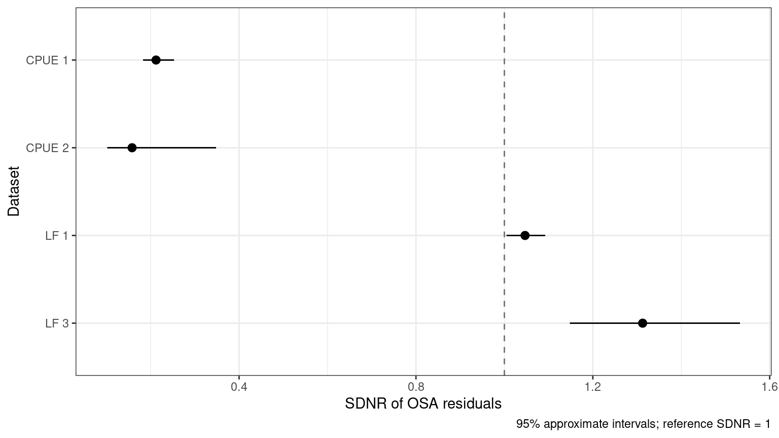

Figure 1: Opakapaka OSA residual SDNR by dataset. The dashed line is one, and the horizontal intervals are approximate 95% intervals. Parameters, including estimated recruitment deviations, are held at their fitted values in this fixed-effects model.

knitr::kable(opal_derived(opaka, "osa")$summary[,
  c("dataset", "family", "n", "sdnr", "lower", "upper", "excluded", "failures")], digits = 3)

dataset	family	n	sdnr	lower	upper	excluded
CPUE 1	lognormal	75	0.212	0.183	0.253	0
CPUE 2	lognormal	7	0.158	0.102	0.348	0
LF 1	multinomial	1103	1.047	1.005	1.092	172
LF 3	multinomial	94	1.313	1.148	1.533	25

SDNR is the standard deviation of normalised OSA residuals. Values above one indicate more residual variation than expected under the fitted observation model; values below one indicate less. This example has relatively small CPUE SDNRs and a larger research-fleet composition SDNR. These are prompts to examine variance assumptions, weighting, and model flexibility. They are not automatic instructions to reweight the data. The chi-squared intervals assume independent normal residuals with known model parameters, so fitted-parameter effects make them approximate.

Each CPUE index has its own row, even when several indices use the same fishery. Length and weight compositions are grouped by fishery. Inspect time patterns and normal quantiles as well as SDNR:

plot_osa_residuals(opaka, type = "qq")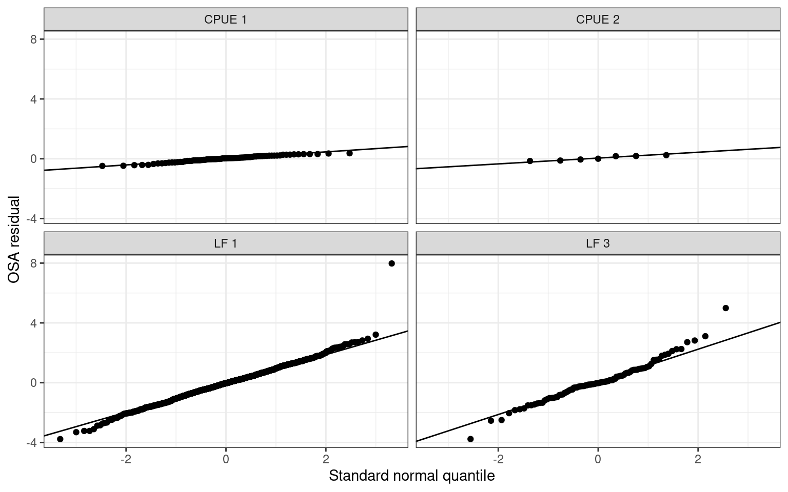

Figure 2: Normal quantile plots for the same OSA residuals.

Likelihood and conditioning conventions

Observation likelihood	Conditional distribution used by OSA
Lognormal CPUE	Normal distribution of log CPUE, with the fitted total log-scale SD
Multinomial composition	Sequential binomial distributions
Dirichlet composition	Sequential beta distributions
Dirichlet–multinomial composition	Sequential beta-binomial distributions

All three composition likelihoods work for both length and weight data. The calculation uses the prepared observations, fitted probabilities, effective sample sizes, and concentration parameters. It introduces no extra pseudocounts. Multinomial rounding follows the likelihood. Discrete residuals randomise within the observed count’s probability mass; an explicit seed makes them reproducible without changing the caller’s random-number state.

For fixed-effect models, residuals condition on the fitted parameters. When the model declares random effects through opal_obj(random = ...), Opal uses RTMB’s sequential, Laplace-based integration of those latent states. Other observation streams remain observed while each stream is processed. This distinction matters for recruitment deviations: estimated fixed effects and integrated random effects are different diagnostic targets.

Within a stream, input order defines observation order, followed by ascending composition bin. The final bin is constrained and has no residual. Removed fisheries, zero sample sizes, exhausted counts, and any numerical failures remain in opal_derived(x, "osa")$residuals with an explicit reason. Failed residuals are reported in the summary; they must not be mistaken for a successful check. Catch is conditioned on, rather than modelled with an observation likelihood, so its reconstruction differences are not OSA residuals. Recruitment priors are also outside this observation diagnostic.

A small, reproducible assessment

The remaining examples use simulated data for two fisheries, 12 years, and two seasons. opal_example_inputs() supplies CPUE and both composition streams; its family argument selects any of the three composition distributions. Three parameters are estimated, and biology and recruitment deviations are fixed. This is a software tutorial, not an assessment of a real stock.

inputs <- opal_example_inputs("multinomial", seed = 712)
assessment <- opal_obj(inputs$data, inputs$parameters, inputs$map)
assessment <- opal_fit(assessment)
summary(assessment)

<opal_obj> fitted
Active parameters: 3
Objective: 240.3783
Fit check: passed  | MCMC check: not run

cpue_data$ts is a one-based, flattened year/season index: (year_index - 1) * n_season + season_index. The first year’s seasons are 1 and 2; the second year’s seasons are 3 and 4. Composition years are model-year indices because their predictions use catch accumulated over that year. data$years gives display labels. Biological vectors are at age unless the model explicitly supplies length-based biology; weight and spawning-output units must be consistent with the supplied inputs. catch_units_f distinguishes weight from numbers. Use plot_catch(weight_units = ...) and plot_biomass_spawning(units = ..., scale = ...) for explicit display units.

Biological acceptance

opal_diagnose(assessment)

$passes
[1] TRUE

$checks
 initial_equilibrium      harvest_penalty           population
                TRUE                 TRUE                 TRUE
           mortality             maturity   spawning_potential
                TRUE                 TRUE                 TRUE
              weight          selectivity            steepness
                TRUE                 TRUE                 TRUE
         recruitment      spawning_output              harvest
                TRUE                 TRUE                 TRUE
           depletion catch_reconstruction
                TRUE                 TRUE

$metrics
$metrics$initial_penalty
[1] 0

$metrics$total_penalty
[1] 0

$metrics$max_harvest
[1] 0.007761073

$metrics$max_relative_catch_error
[1] 5.636512e-11

A passing fit requires convergence, the gradient and Hessian checks, parameter bounds, and biological feasibility. The latter includes initial-equilibrium and harvest penalties, abundance, mortality, maturity, spawning potential, harvest fractions, catch reconstruction, and depletion. Positive continuation keeps an invalid trial state numerically evaluable; a positive penalty does not establish a valid equilibrium.

Posterior checking evaluates every retained joint draw, including its bounds and draw-specific biology, in addition to R-hat, ESS, divergences, and tree depth. Failures retain their chain, iteration, and reason. Marginal draws that omit random effects cannot pass the full biological posterior check. Old validation records become stale when the validation contract changes.

Other composition distributions

These examples fit both composition streams for each likelihood, then collect the same SDNR statistic. The seed controls independent simulated observations and residual randomisation; results need not be identical across distributions.

family_diagnostics <- lapply(c("multinomial", "Dirichlet", "Dirichlet-multinomial"), function(family) {
  z <- opal_example_inputs(family)
  fit <- opal_fit(opal_obj(z$data, z$parameters, z$map))
  fit <- opal_osa(fit)
  out <- opal_derived(fit, "osa")$summary
  out$composition_family <- family
  out
})
knitr::kable(do.call(rbind, family_diagnostics)[,
  c("composition_family", "dataset", "n", "sdnr", "failures")], digits = 3)

composition_family	dataset	n	sdnr
multinomial	CPUE 1	24	0.898
multinomial	CPUE 2	24	1.062
multinomial	LF 1	24	0.734
multinomial	LF 2	24	0.926
multinomial	WF 1	24	1.239
multinomial	WF 2	24	0.935
Dirichlet	CPUE 1	24	0.895
Dirichlet	CPUE 2	24	1.064
Dirichlet	LF 1	24	0.641
Dirichlet	LF 2	24	0.827
Dirichlet	WF 1	24	1.141
Dirichlet	WF 2	24	0.774
Dirichlet-multinomial	CPUE 1	24	0.898
Dirichlet-multinomial	CPUE 2	24	1.062
Dirichlet-multinomial	LF 1	24	0.864
Dirichlet-multinomial	LF 2	24	0.944
Dirichlet-multinomial	WF 1	24	0.998
Dirichlet-multinomial	WF 2	24	1.001

plot_composition(assessment, type = "lf", fishery = 1)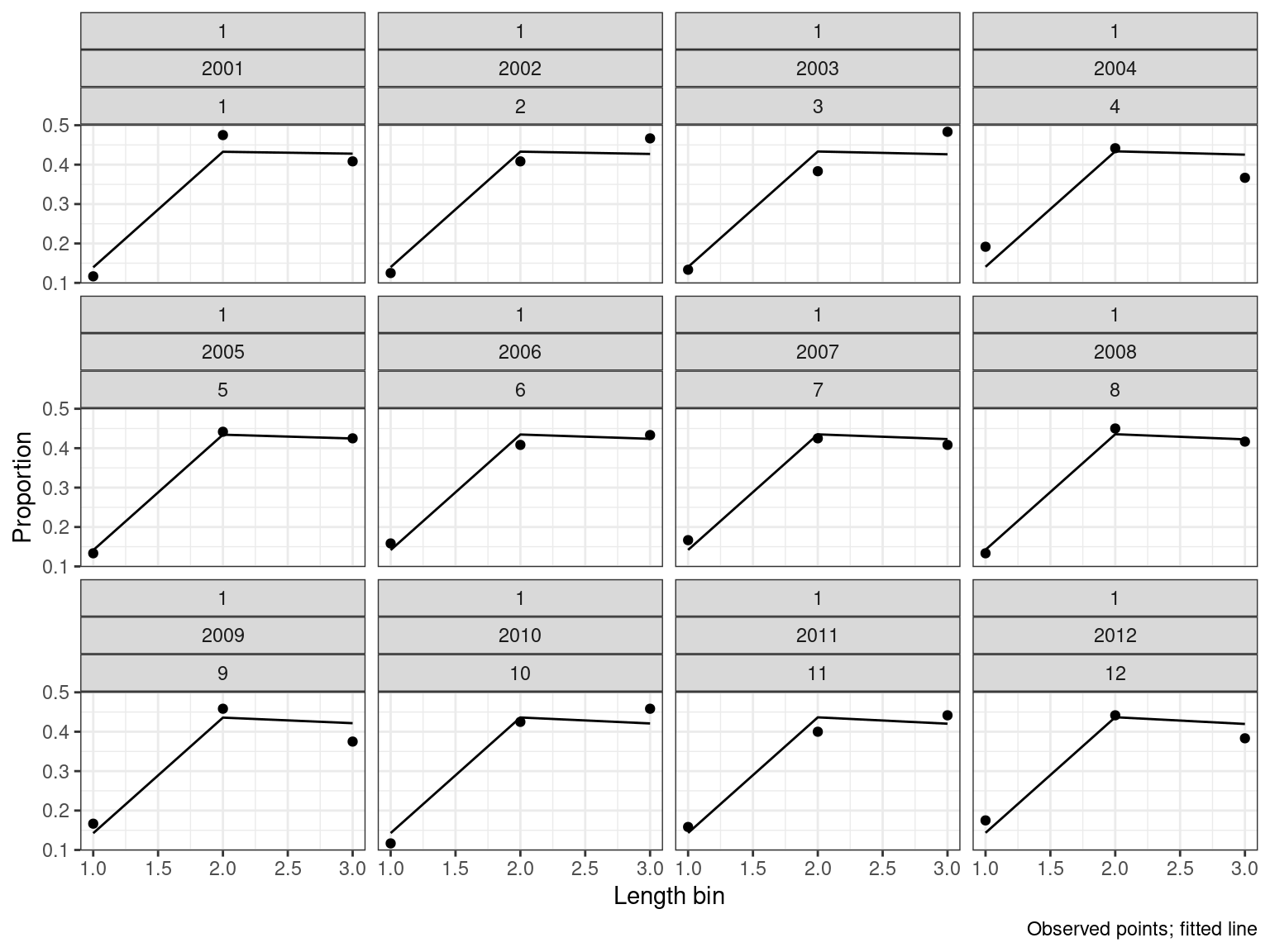

Figure 3: Observed length-composition proportions and fitted probabilities for the first fishery in the simulated example.

Posterior analysis

The bundled simulated posterior was generated with four chains, 1,000 warm-up iterations, and 1,000 retained iterations per chain. Its generation script is data-raw/generate-assessment-example.R. That script requires both fit and MCMC checks to pass before saving. Website builds read the result instead of sampling. To reproduce it yourself:

assessment <- opal_mcmc(assessment, seed = 927, chains = 4, cores = 1,
                       num_warmup = 1000, num_samples = 1000, adapt_delta = 0.95)
assessment <- opal_check(assessment, "mcmc")
opal_save(assessment, "simulated-assessment.rds")

sampled <- opal_read(system.file("extdata", "assessment_example.rds", package = "opal"))
# Refresh diagnostics under the current validation version without resampling.
sampled <- opal_check(sampled, "fit")
sampled <- opal_check(sampled, "mcmc")
summary(sampled)

<opal_obj> sampled
Active parameters: 3
Objective: 240.3783
Fit check: passed  | MCMC check: passed
MCMC: 4 chains; 1000 retained iterations

knitr::kable(sampled$validation$mcmc$metrics$parameters, digits = 3)

variable	rhat	ess_bulk	ess_tail
log_B0	1.000	4087.463	3059.671
log_cpue_q[1]	1.000	3882.720	2788.743
log_cpue_q[2]	1.001	5052.341	3327.968

sampled$validation$mcmc$metrics$biology[c("passes", "checked", "scope")]

$passes
[1] TRUE

$checked
[1] 4000

$scope
[1] "all retained joint draws"

Summaries use each draw’s own model report and preserve the selected chain and iteration identifiers. Non-finite values stop the calculation rather than being silently removed. Running summaries does not turn an unchecked posterior into an accepted one.

sampled <- opal_posterior(sampled,
  quantities = c("B0", "spawning_biomass_y", "static_depletion_y"))
posterior <- opal_derived(sampled, "posterior")
knitr::kable(posterior$parameters, digits = 3)

quantity	element	mean	sd	q0.025	q0.500	q0.975	parameter
parameter	1	11.476	0.280	10.953	11.467	12.041	log_B0
parameter	2	-0.234	0.026	-0.285	-0.234	-0.183	log_cpue_q[1]
parameter	3	0.176	0.026	0.125	0.176	0.228	log_cpue_q[2]

depletion <- subset(posterior$reports, quantity == "static_depletion_y")
depletion$year <- c(sampled$data$years, sampled$data$last_yr + 1)
ggplot2::ggplot(depletion, ggplot2::aes(x = year, y = q0.500)) +
  ggplot2::geom_ribbon(ggplot2::aes(ymin = q0.025, ymax = q0.975), alpha = 0.2) +
  ggplot2::geom_line() + ggplot2::labs(x = "Year", y = "Spawning output / unfished output") +
  ggplot2::theme_bw()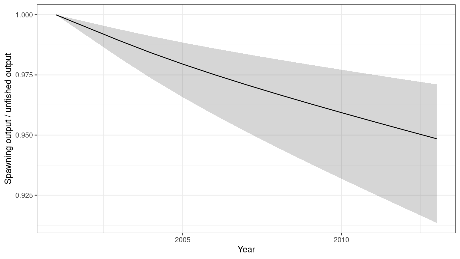

Figure 4: Median and 95% posterior intervals for simulated depletion. These intervals are conditional on the model’s fixed biology and recruitment deviations.

plot_prior_posterior(sampled)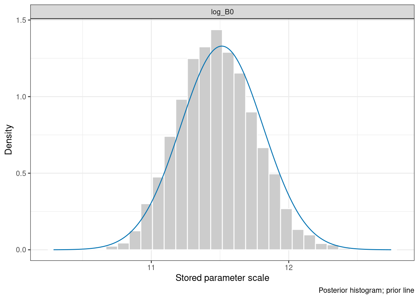

Figure 5: Specified log-spawning-output prior and the simulated example’s posterior. Densities are on the stored parameter scale.

The plotted prior is its specified, untruncated density; bounds may further restrict the target. Shared-map parameters with multiple prior contributions are omitted with a warning rather than displayed as a misleading single prior. SparseNUTS diagnostics can use opal_as_tmbfit(sampled) for additional chain plots.

Profiles and model grids

opal_profile() fixes a parameter value and re-optimises the remaining active parameters. It profiles the penalised objective, including priors, unless those terms are absent. Do not interpret it automatically as a likelihood-ratio confidence interval. Inspect the saved convergence, gradient, biological checks, and component contributions for every point.

centre <- assessment$fit$parameters$log_B0
assessment <- opal_profile(assessment, "log_B0", centre + seq(-0.5, 0.5, length.out = 9))
knitr::kable(opal_derived(assessment, "profile")$table, digits = 3)

value	objective	delta	passes	error
10.960	241.965	1.586	TRUE	NA
11.085	241.251	0.873	TRUE	NA
11.210	240.759	0.381	TRUE	NA
11.335	240.472	0.094	TRUE	NA
11.460	240.378	0.000	TRUE	NA
11.585	240.470	0.091	TRUE	NA
11.710	240.740	0.362	TRUE	NA
11.835	241.186	0.807	TRUE	NA
11.960	241.803	1.425	TRUE	NA

plot_opal_profile(assessment)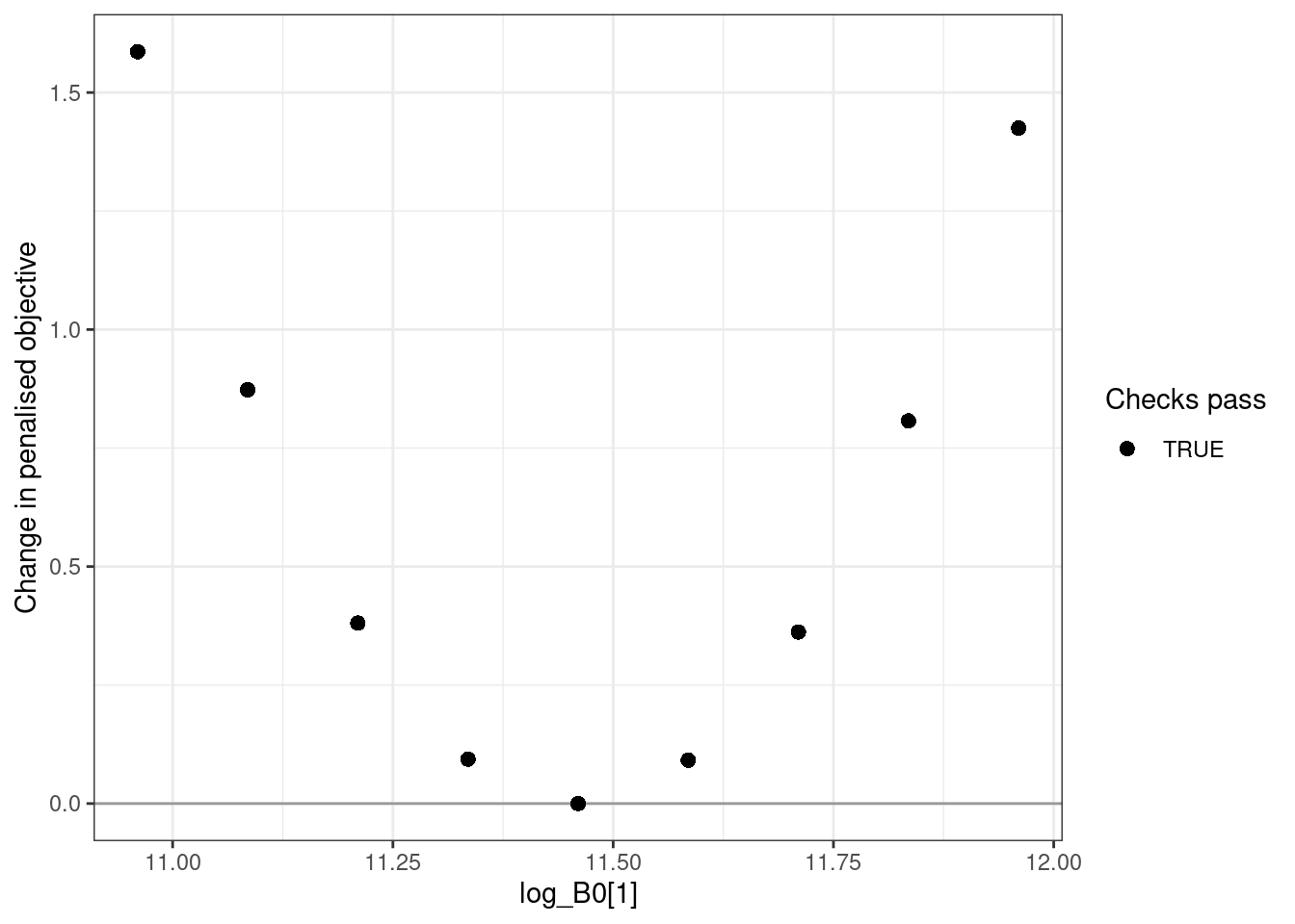

A grid makes alternative assumptions explicit. Checkpoints are reusable only when the scientific target, starting state, fitting controls, and validation contract match. Failed scenarios remain in the result.

higher_mortality <- inputs$data
higher_mortality$M <- rep(0.35, inputs$data$n_age)
grid <- opal_grid(opal_obj(inputs$data, inputs$parameters, inputs$map),
  scenarios = list(base = list(), higher_M = list(data = higher_mortality)))
knitr::kable(grid$summary, digits = 3)

model	objective	passes	reused	error
base	240.378	TRUE	FALSE	NA
higher_M	257.592	TRUE	FALSE	NA

For a larger analysis, supply directory = "sensitivity-checkpoints". Sampling and balanced model selection are explicit subsequent steps:

grid <- opal_grid_mcmc(grid, seed = 927, chains = 4, cores = 4,
                       num_warmup = 1000, num_samples = 1000)
selection <- opal_grid_draws(grid, n_per_model = 400, seed = 123)

Balanced selection requires a current passing posterior check for every grid member. It samples without replacement, balances chains, and attaches equal model weights. Equal model weights are a scientific assumption, not a conclusion from comparing the fitted objectives.

Equilibrium reference points

opal_msy() calculates deterministic equilibrium yield using a stated fleet allocation, fixed reference-year selectivity, and Beverton–Holt recruitment. Here the fleets receive equal harvest-intensity weights. This calculation is independent of the projection engine.

assessment <- opal_msy(assessment, fleet_weights = c(0.5, 0.5))
knitr::kable(opal_derived(assessment, "msy")$draws, digits = 3)

iteration	chain	draw	msy	b_msy	r_msy	u_msy	depletion_msy	terminal_b_bmsy	at_upper_bound	resolved
NA	NA	1	2123.869	27020.71	3509.737	0.16	0.285	3.329	FALSE	TRUE

u_msy is a scalar seasonal harvest intensity, not an instantaneous annual fishing mortality. Fleet/age harvest fractions are u * fleet_weight[f] * selectivity[f,a]. Yield uses model weight units, while b_msy uses model spawning-output units. The engine matches the historical seasonal survival and plus-group convention and solves equilibrium recruitment without recruitment deviations or positive continuation. Upper-bound maxima are flagged as unresolved.

# Deliberately small, balanced subset for a quick tutorial calculation.
selected <- unlist(lapply(0:3, function(chain) chain * 1000 + seq(1, 901, by = 100)))
sampled <- opal_msy(sampled, fleet_weights = c(0.5, 0.5),
                    uncertainty = "mcmc", draws = selected)
msy <- opal_derived(sampled, "msy")
knitr::kable(head(msy$draws), digits = 3)

	iteration	chain	draw	msy	b_msy	r_msy	u_msy	depletion_msy	terminal_b_bmsy	at_upper_bound	resolved
1	1001	1	1	2288.590	29116.36	3781.941	0.16	0.285	3.342	FALSE	TRUE
101	1101	1	101	1866.202	23742.57	3083.936	0.16	0.285	3.303	FALSE	TRUE
201	1201	1	201	2429.690	30911.48	4015.111	0.16	0.285	3.352	FALSE	TRUE
301	1301	1	301	2227.596	28340.37	3681.148	0.16	0.285	3.337	FALSE	TRUE
401	1401	1	401	1780.616	22653.70	2942.503	0.16	0.285	3.293	FALSE	TRUE
501	1501	1	501	1491.058	18969.84	2464.004	0.16	0.285	3.251	FALSE	TRUE

msy$probability_below_bmsy

[1] 0

Every selected draw supplies its own biology. This 40-draw result demonstrates the calculation; use an appropriately sized posterior analysis for inference. These reference points are conditional on the fleet mix, selectivity, biology, and deterministic recruitment assumptions. They are not stochastic MSY or management advice.

Projection development, estimated selectivity time blocks, and close-kin components are outside the scope of this tutorial and feature addition.